I recently had the task to optimize a ray tracing algorithm in hardware on an FPGA and remembered the “Fast Inverse Square Root” – that has been used to accelerate rendering for Quake 3. So I studied the math behind the FISR and found a gigantic world of very precise and fast approximations using logarithms.
- The Idea
- Floating Point Representation
- Division: Order 1 – Approximation
- Higher Order Approximations
- Offset Compensation
- Rule Them All
The Idea
First, what is the Idea behind those logarithmic approximations?
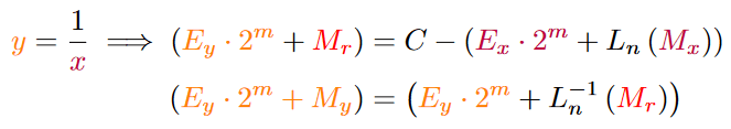
If we, for example, want to have a faster approximation for the inverse of a number – because computers need a long time to divide – and look at the following equation:

And take the binary logarithm of that equation:
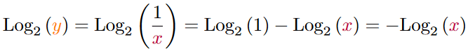
We can see that no longer a division is needed and we only need to negate the number. So now the question becomes, can we find a nice approximation for the logarithm. And since we are in comuting, lets find one that exploits floating point numbers.
Floating Point Representation
A floating point number has a signed bit, a field for the exponent and a field for the mantissa, as shown in the following bitfield:
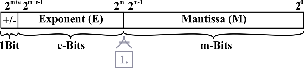
In the binary something happens, that happens in no other base. The number before the comma will always be a one and thus holds no information and does not need to be stored in the bitfield. For all further calculations, we will assume that the number is positive and the signed bit will be zero.
If we were to describe a positive floating point number in its bitfield and number representation it would look like this:
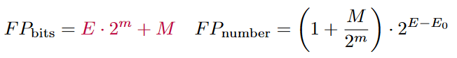
You might wonder where the E0 is coming from? The exponent field in a floating point number is always a positive integer that is implicitly subtracted by an offset to also represent negative exponents.
If we now look at the logarithm of the floating point number we can see that something very interesting happens:
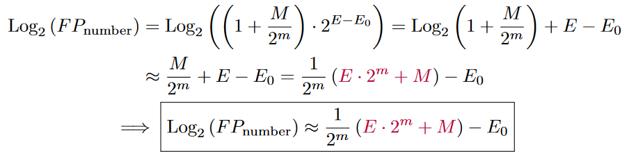
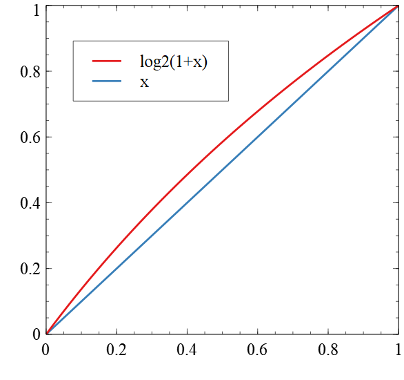
So, in some sense, the logarithm of a number already is the floating point representation of that number! But why does this approximation work? The mantissa of a floating point number can only represent a number between zero (including) and one (excluding). We only have to find a good approximation for the logarithm from zero to one. And Log2(1+x) is approximately x. The error in this example is always positive. Later we will also take the error offset into account and distribute the error around zero.
Division: Order 1 – Approximation
Now that we know, that the logarithm of a function is in some sense its own floating point representation, we can solve the initial division.
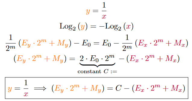
Low and behold we have replaced a division, that can take up to 48 clock cycles to compute and replaced it by a simple subtraction that only takes 1 clock or zero clock cycles if combined with other operations. Isn’t this exciting?
Try it in Yourself
Let’s look at our results in a coding example in “Compiler Explorer”. It lets you write, compile and run code online: Code: Fast Division Order: 1
inline float approx_inverse_O1(float a){
    const unsigned int C= (1 << (23 /*mantissa bits*/ +1)) * 127 /*exponent offset*/;
    return std::bit_cast<float>(C -  std::bit_cast<unsigned int>(a));
}
If you cannot see the output generated, then click on the gear-wheel above the compiler/assembly and select “Execute the code”. The results of the approximation is exact for all values that can be represented by a power of two. We have an error of only 6.8% and a squared error of 0.63%. For replacing a division by a simple subtraction this is already a really good result.
In the following, I also want to show how we can find higher-order approximations to get better and more precise approximations as well as expand this type of approximation to cover a wide variety of mathematical functions.
Higher Order Approximations
There are two parts to finding a better approximation. The first is a better approximation for entering the logarithmic world and the second one is to leave the logarithmic world. Let’s start by finding better higher-order approximations for the logarithm. Let’s start by rewriting the equation above by replacing M with L(M) and then define the approximation function L later.

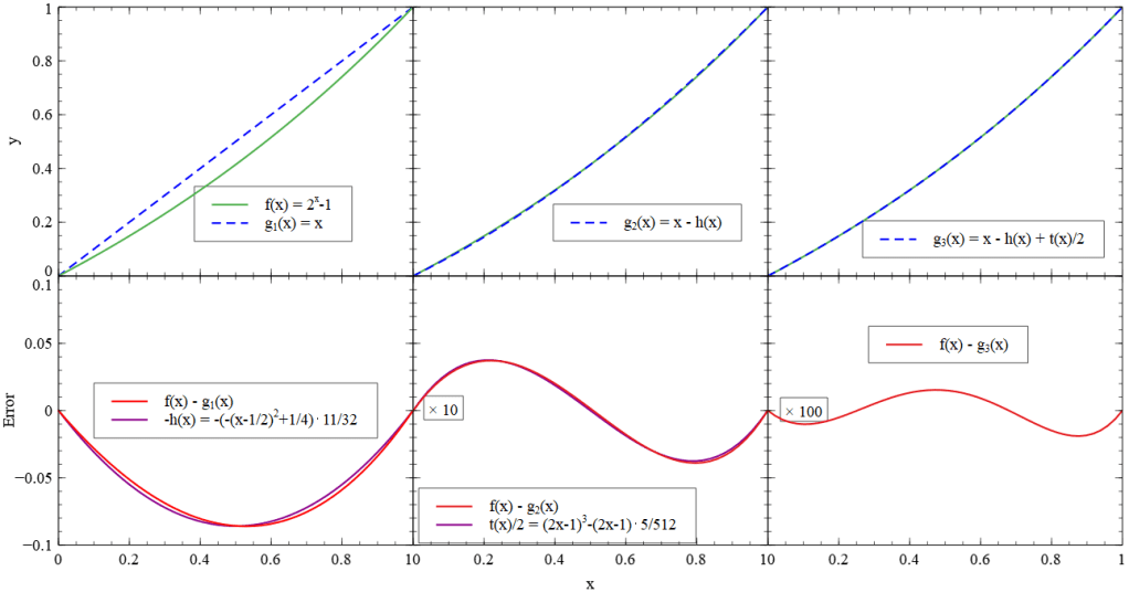
In the following diagrams, you can see the logarithm and its approximation in the first row and the error in the second row. In the left column, you can see the approximation that we already used in the calculations above. I tried to approximate the error with a quadradic function and then added it in the next step which you can see in the middle. The same has been done to find a third-order approximation. Notice that the second and third y-axis of the error function has been multiplied by 10 and 100 to display the error.
Approximating the Logarithm
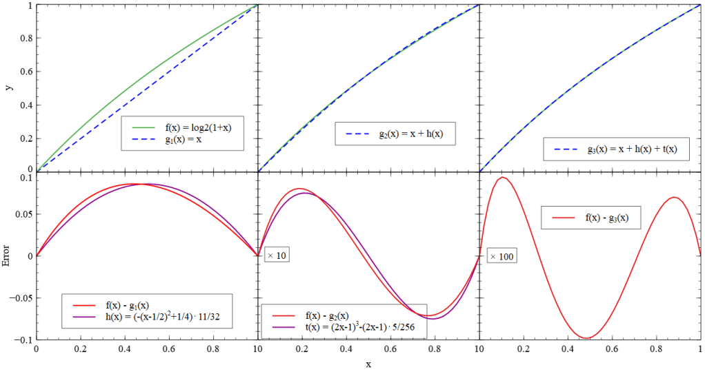
You might wonder why I chose 11/32 and 5/256 as a gain in h(x) and t(x). This is because a division by any power of two can be implemented as bitshift operations. In hardware those bitshifts are just wires, so they do not really need time or resources.
From this, we can derive approximations for the logarithm of the Mantissa. Here and there, I evened out the numbers to get smaller coefficients:
Approximating the Exponent
From the equation above, where we replaced Mx by L(Mx) we can use the functions found above to replace the right-hand side. However, if we calculated the right side of the equation, what we have is the result, but with the L function still applied to the mantissa. So we need to apply the inverse of L to the mantissa to get the real result. Therefore we need to approximate the exponent instead of the logarithm.
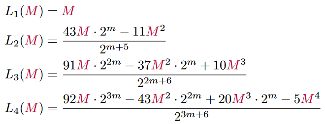
And thus the approximations for the inverse logarithms of the mantissa look like:

I tried to find approximations, that have relatively small coefficients and are all divisible by a power of two which can be replaced by a bitshift. With this, we can now describe the logarithmic approximation as a system of two equations:
Try it Yourself
You can try the approximation in code following this link to the “Compiler Explorer” Code: Approx Inverse – O1, O2, O3 and O4. When you execute the code, you can see that with each increasing order of approximation, the error and standard deviation gets smaller by a factor of 10, also seen in the following table.
| K = 0 | O1 approximation | O2 approximation | O3 approximation | O4 approximation |
| mean error | 0.0568528 | 0.000238133 | 2.27909e-05 | 8.31896e-06 |
| standard deviation | 0.0256817 | 0.00402364 | 0.000374827 | 4.32418e-05 |
In the above table the absolute mean error can be observed for 220 uniform samples from an input range of x = [1.0, 2.0] and an output range of y = [1.0, 0.5].
Rendering Exaple
Let us now have a look at what those numbers of the “mean error” and “standard deviation” actually mean. So that we can have a more intuitive understanding of the approximation result. In the following, together with my study colleagues – Timoty Grundacker and Oliver Theimer – we have implemented that approximation for the reflections of a 3D Ray-Traceing renderer


Right: Order 1 Approximation
μ = 0

Right: Order 2 Approximation
μ = 0


Right: Order 3 Approximation
μ = 0
In the comparison above, one can see, that the offset from the table above corresponds with the size difference of the reflections. In the next chapter I will show how to compensate the mean error.
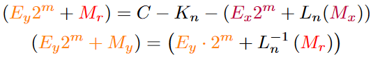
Offset Compensation
The mean error can be turned close to zero by adding and subtracting an offset to the constant C. That offset can be aquired by calculating the error integrals over the approximation functions, or using a binary numeric optimizer.
Try it yourself
In this code example the offset – found by an optimizer – has been applied with the following results:
| K != 0 | O1 approximation K = 982606 | O2 approximation K = 4159 | O3 approximation K = 398 | O4 approximation K = 145 |
| mean error | 2.32831e-08 | 4.23752e-08 | -4.55475e-09 | 1.41072e-08 |
| mean squared error | 0.0229683 | 0.00398216 | 0.000373397 | 4.23408e-05 |
In the above table the absolute mean error can be observed for 220 uniform samples from an input range of x = [1.0, 2.0] and an output range of y = [1.0, 0.5]. You can see that the mean error is way smaller than before and almost zero compared to the previous example where the offset has not been compensated. However, the standard deviation stays unchanged.
In the following you can see a comparison of the amount of hardware that has been estimated for each operation in the FPGA:
| Divider | O1 Approx Divider | O2 Approx Divider | O3 Approx Divider | |
| LUTs | 2825 | 32 | 648 | 1048 |
| Pipeline Steps | 48 | combinatorical or 1 | 8 | 12 |
Rule Them All
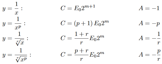
Now that we have solved it for one equation, we can use it for all equations and rule the world …. hahahaha! No seriously, since this is a logarithmic approximation we can use this now to approximate all multiplicative functions, as well as special math functions like – of course – exponents and logarithms. The approximation functions L(M) can be used to select the precision, speed or computation size.
The algorithm from above can now be parameterised by the constant C that we get from taking the logarithm and the operator A.
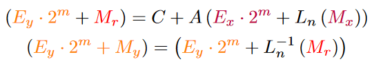
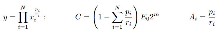
Here are the parameters for some common math operations that usually take long to compute and benefit from this approximation:
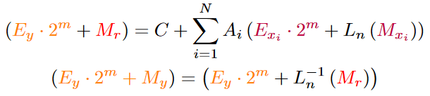
In a more generalised form, the approximation algorithm looks like this:
Now that you are equipped with this kind of algorithm, imagine how you could change the world.
- You could accelerate Machine Learning (ML) and its big matrix multiplications by approximating all multiplications with an order 1 addition. One may argue that the error is irrelevant here because the ML-Network probably learns it anyway.
- Accelerate real-time systems. What is more important when your self-driving car is about to crash into a wall? Reacting faster or reacting more precise?
- Accelerate media that is consumed by humans like 3D Graphics or Audio. As long as one does not hear or see the difference, the approximation is good enough.
- And if you truly want to be crazy, then you could even recursively approximate all remaining multiplications of the higher-order approximations. So that everything ends up being shifts and additions. That would probably introduce a larger error. But on the upside higher order approximations get another speed boost and need less hardware. When you take on this challenge, please let me know about your findings.

Leave a comment